SARSA Hedging Model

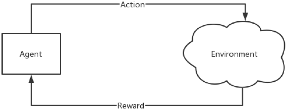
Continuous rebalancing is an idealization. Real portfolios change at discrete intervals, and complex structured products make hedging more difficult. This study treats the hedge as a sequence of decisions learned through interaction with a simulated market.

The case study uses a structured note with conditional coupons and an autocall feature. Coupons depend on the underlying price clearing an interest barrier; the note can redeem early when its autocall condition is met. This path-dependent payoff provides a more complex hedging problem than a simple buy-and-hold equity position.

The experiment uses SARSA, an on-policy reinforcement learning algorithm, to learn a hedging strategy for a Phoenix option. Its reward reflects the portfolio’s Sharpe ratio, incorporating risk as well as return. The framework also considers different weights for intermediate and terminal outcomes.

The agent holds one Phoenix option and adjusts its underlying-equity position at monthly observation dates. Its state has three variables: the underlying price, time to maturity, and current equity position. Prices follow geometric Brownian motion; short selling and borrowing or lending at the risk-free rate are allowed in the simulation.

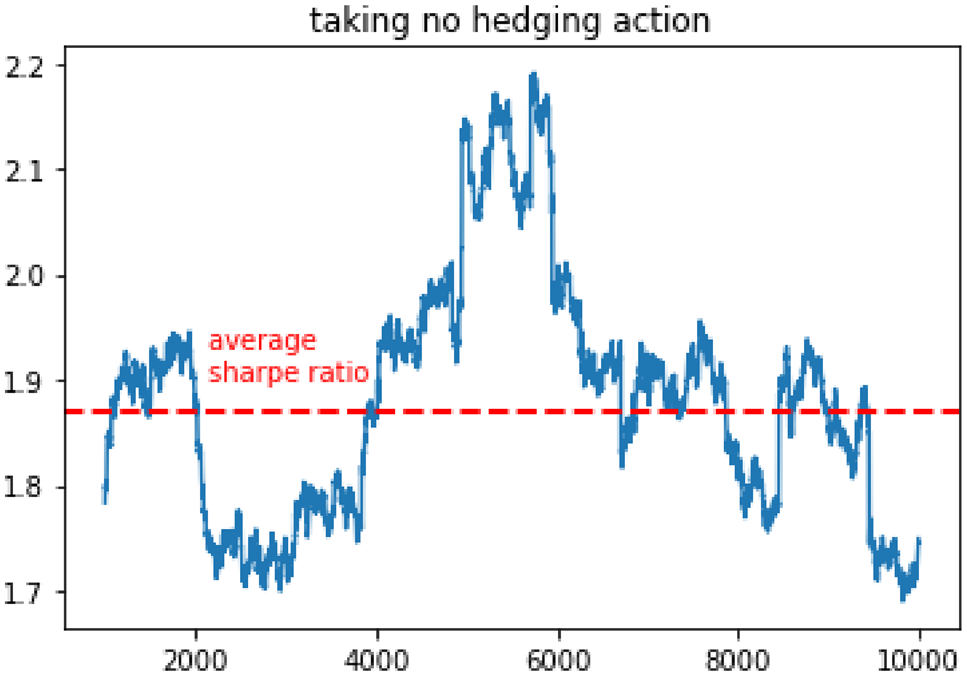
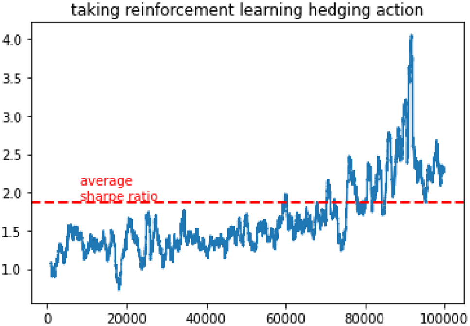
The example has a 12-month term, monthly coupon observations, quarterly autocall observations, an 80% interest barrier, a 3% risk-free rate, and 15% underlying volatility. A decaying epsilon-greedy policy shifts the agent from exploration toward exploiting its Q-table. The benchmark averages 10,000 unhedged simulations; the agent is then trained over 100,000 price paths.

The Q-table is updated from the current state and action, the next reward, and the next state–action pair: Q(s,a) ← Q(s,a) + α[r + γQ(s′,a′) − Q(s,a)]. Because SARSA uses the action actually selected by the current policy, exploration also affects the value estimates. When a state has not previously appeared in the table, the implementation defaults to taking no hedging action.

The reward multiplies the portfolio’s running Sharpe ratio by a time-dependent weight. With τ denoting months remaining, the baseline weight is (12 − τ) / [12(τ + 1)]. This makes the terminal outcome more influential while retaining feedback during the holding period. The option’s value within the portfolio is estimated using Monte Carlo simulation.

In the reported simulations, the learned strategy achieved a higher Sharpe ratio at maturity than holding the product without hedging. The unhedged benchmark is 1.87 in this setup. Learning is uneven: the paper reports performance below the benchmark until about 75,000 episodes. These values describe this particular simulation, not expected market returns.

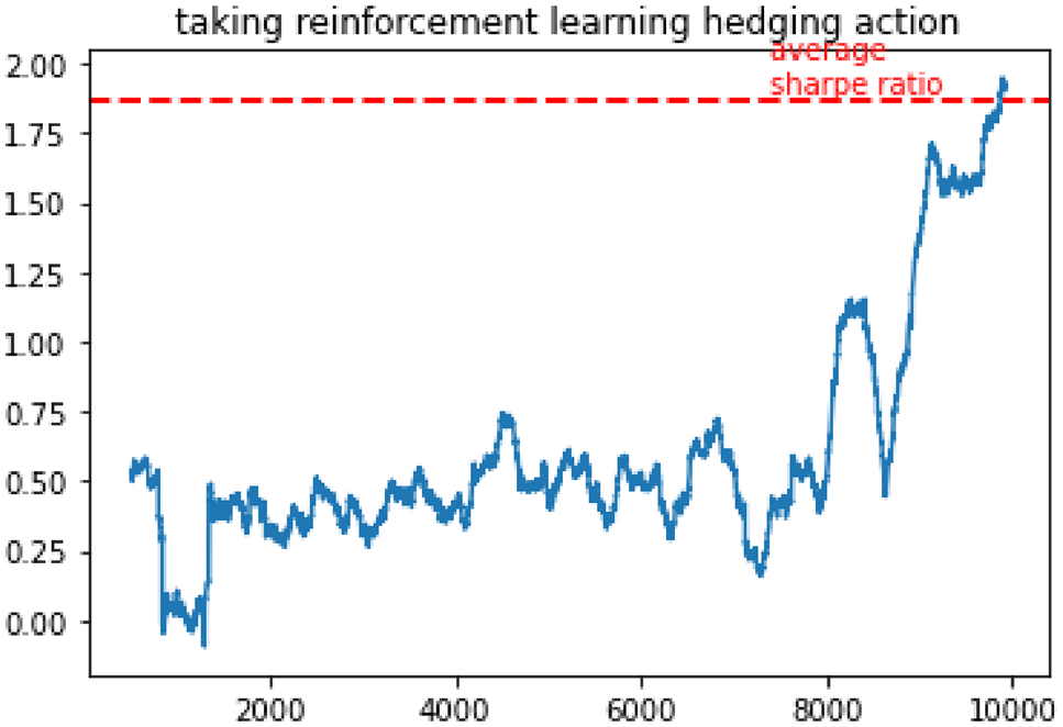
Section 6.1 changes the weight to (12 − τ) / [12(5τ + 1)]. Both weights reach 1 at maturity, but the alternative suppresses earlier rewards more strongly. The paper reports crossing the unhedged benchmark in fewer than 10,000 iterations in this experiment, compared with roughly 75,000 episodes in the earlier setup. This illustrates sensitivity to the objective, rather than a general convergence guarantee.

The discussion proposes replacing the Sharpe ratio with the Sortino ratio to emphasize downside risk, or using a mean–variance utility function to encode risk aversion. It also discusses DQN as a possible alternative to a growing Q-table. These are extension directions: the paper does not report a head-to-head empirical comparison of SARSA, Q-learning, and DQN.

The evaluation uses simulated data, not live trading results. The paper identifies growth of the Q-table as a computational limitation and discusses alternative learning algorithms and reward measures as directions for further work.